Uncertainty Quantification in Nuclear Engineering Thermal-Hydraulics

Before continuing the discussion of uncertainty analysis of code predictions, this section defines some additional terminologies to avoid later confusion.

The notion of simulator introduced in Computer Simulation and Safety Analysis of Nuclear Power Plant is depicted in a more generic way, as an input/output model in Fig. 3.

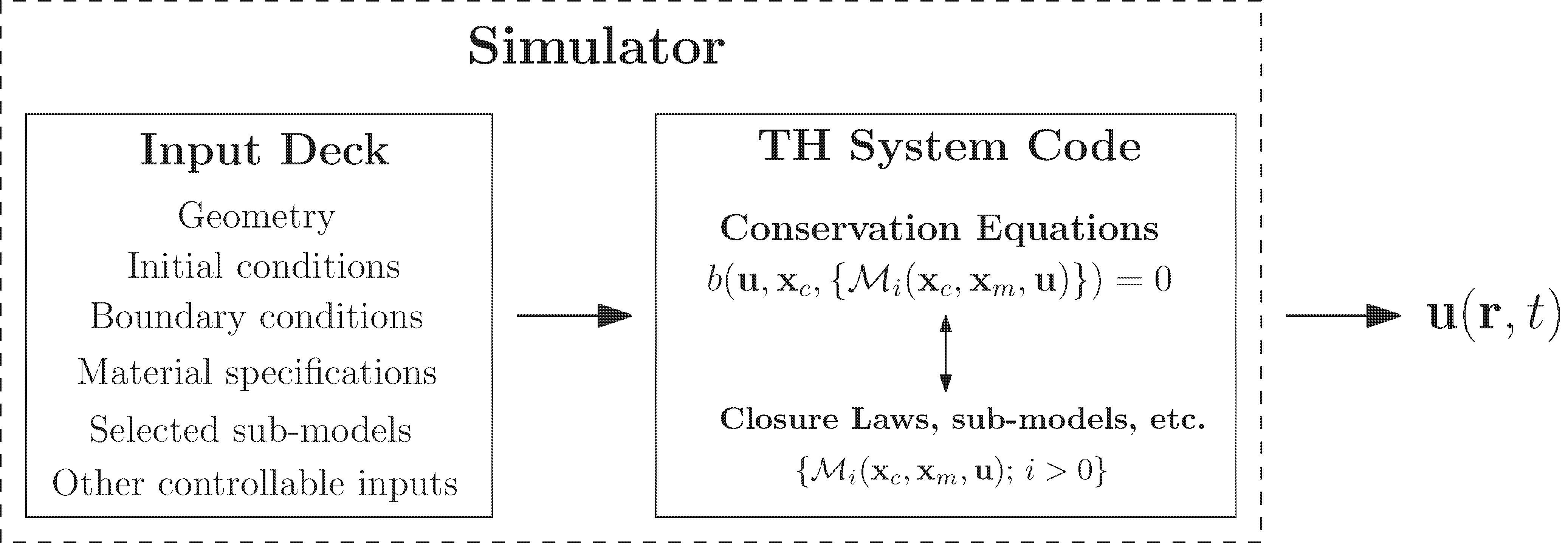
Fig. 3 Simplified illustration of a simulator as an input/output model.

The input deck defines a specific problem (i.e., system) of interest and can be seen as the input of TH codes. It includes the geometrical configuration (i.e., the nodalization), the material and fluid involved, the initial and boundary conditions, and possibly the settings for the numerical solver. Some of these specifications (such as the boundary conditions) are parametrized and constitutes controllable inputs denoted by \(\boldsymbol{x}_c\). The simulator is to be run for a given controllable input value [*]. The conservation equations of the code are closed with additional set of closure laws (and other sub-models) \(\mathcal{M}_i(\boldsymbol{x}_c, \boldsymbol{x}_m, \boldsymbol{u})\). These closure laws are, in turn, parametrized by a set of model specific parameters denoted by \(\boldsymbol{x}_m\) which are referred to as the physical model parameters. Both the controllable inputs and the physical model parameters are considered by the code as inputs.

Specifying the input deck, as far as the user is concerned, completely defines the problem and the code solves the conservation equations \(b\) (Fig. 3) to estimate the physical variables \(\boldsymbol{u}(\boldsymbol{r}, t)\) (where \(\boldsymbol{r}\) and \(t\) denote space and time variables, respectively) associated with the fluid flow and heat structure (e.g., fluid pressure, temperature, wall temperature, etc.). These “raw” outputs are further post-processed to obtain relevant QoIs for the problem at hand (e.g., max. temperature, max. pressure, onset time, etc.).

Forward Uncertainty Quantification

Best-estimate analysis attempts to describe as realistically as possible the behaviors of the physical processes that occur during a plant transient. And yet, neither complete understanding nor enough data is always available to adequately simulate these complex physical phenomena. Simplifying assumptions, approximations, and expert judgments remain to some degree unavoidable for a complete analysis.

Hence, best-estimate analysis has to be complemented with uncertainty analysis. The ultimate goal of uncertainty analysis is to associate code prediction a with its uncertainty. These combined quantities are then compared with safety limits (e.g., PCT) to check whether the limits still fall outside the uncertainty band of the code prediction.

There are several known sources of uncertainty that render the prediction on \(\boldsymbol{u}(\boldsymbol{r},t)\) and its derived quantities uncertain. The sources of primary interest in the present research are:

1. Uncertainty associated with the controllable inputs. In the case of a controlled experiment, controllable inputs are observed and controlled for. However, their observations might contain errors due to instrument imprecision or inherent variability. When simulating a real accident scenario in a plant, plant parameters prior to the accident scenario can also be measured and constitute uncertain controllable inputs. In addition, parameters defining the accident scenario, such as the break size in a LOCA, or the availability and performance of safety systems can also be treated as uncertain controllable inputs [IAEA02].

2. Uncertainty associated with the physical model parameters. The value of the physical model parameters are often not known a priori. Thus, the uncertainties are epistemic. They can either be estimated using data from a calibration experiment or by expert judgment.

3. Uncertainty associated with the physical models. The physical models themselves are still approximations, even with perfectly known model parameters. If derived in a fully mechanistic manner, some important processes might be unaccounted for due to the inherent complexity and lack of knowledge (i.e., the case of missing physics). On the contrary, if derived fully empirically, models might be derived separately for different elementary processes, while in the applications of the code multiple such models are used in concert. Despite each being validated, it is fair to question the validity of models used in an ensemble. Any of the two tends to cause a systematic bias on the code prediction, the extend of which is unknown and uncertain. As a result, this source of uncertainty is referred to as model bias, inadequacy, or discrepancy.

In uncertainty analysis, the controllable inputs and physical model parameters are modeled as random variables (\(\boldsymbol{\mathcal{X}}_c\) and \(\boldsymbol{\mathcal{X}}_m\), respectively) equipped with probability density functions (PDFs). By transforming the random variable inputs, the simulator output becomes random variable as well

\[\boldsymbol{\mathcal{U}}(\boldsymbol{r}, t) = f(\boldsymbol{\mathcal{X}}_c, \boldsymbol{\mathcal{X}}_m;\boldsymbol{r}, t)\]

where \(f\) represents the simulator as a mathematical function. The QoI related to the random outputs can be summarized by different integral quantities. For instance, the mean of a QoI given by function \(g\) is

\[\mathbb{E}[g] = \int\limits_{\mathbf{X}_c,\mathbf{X}_m} g(f(\boldsymbol{x}_c, \boldsymbol{x}_m;\boldsymbol{r}, t)) \, p(\boldsymbol{x}_c, \boldsymbol{x}_m) \, d\boldsymbol{x}_c \, d\boldsymbol{x}_m\]

where \(p(\boldsymbol{x}_c, \boldsymbol{x}_m)\) denotes the joint PDF for the input parameters.

Using Monte Carlo (MC) techniques, samples are generated from the joint input parameters distribution and are used to run the code multiple times. Afterward, the resulting code outputs (raw or post-processed), are summarized to obtain the uncertainty measure of the prediction. In other words, the uncertainties in the controllable inputs and physical model parameters are propagated forward through the code to quantify the uncertainty of the predictions as shown in Fig. 4. The practice of propagating parametric uncertainty by MC is widely accepted in the nuclear engineering thermal-hydraulics community [LLLANL+90][GHKS94][Wal07][Gla08].

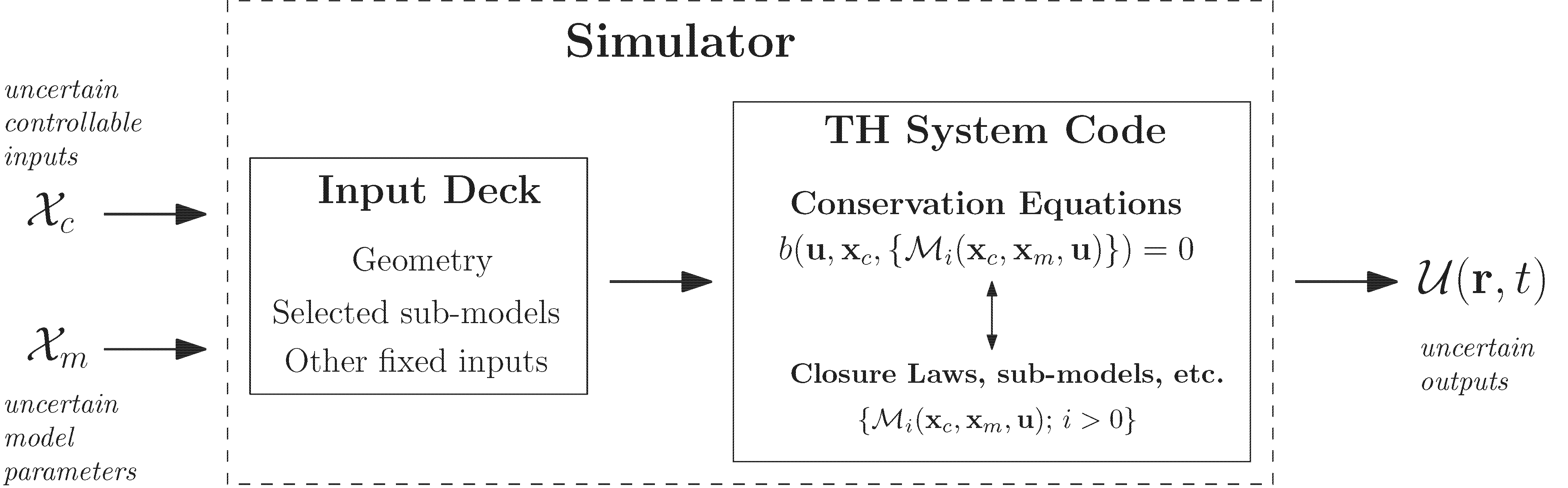
Fig. 4 Simplified flowchart of forward uncertainty quantification of a simulator prediction. Notice that the simulator has been parametrized by the controllable inputs and physical model parameters, each of which are represented as a random variable.

[*]	Later on, controllable inputs correspond to the parameters whose counterparts in a physical experiment which can be controlled by the experimentalist.